Interactive time series in R with dygraphs

Package

The `dygraph` function

The dygraphs package allows creating interactive time series charts in R based on the dygraphs JavaScript library. The charts display the values when hovering over them and allow zooming selecting an area with the mouse (double click to reset the zoom).

The dygraph function takes a time series object, such as a ts or an xts object. In this tutorial we are going to use the ldeaths data set, which contains the monthly deaths from lung diseases in the UK between 1974 and 1979.

# install.packages("dygraphs")
library(dygraphs)

dygraph(ldeaths)

Range selector

The dyRangeSelector function adds a range selector under the chart, which allows selecting the period to display dragging its edges. You can set the initial period with the dateWindow argument, such as dateWindow = c("1976-01-01", "1978-12-01").

dygraph(ldeaths) |>
  dyRangeSelector()

Multiple series

If you pass an object with several time series a line will be drawn for each one. In this example we are binding the deaths of men (mdeaths) and women (fdeaths) with cbind. The colors are set with the colors argument of dyOptions.

deaths <- cbind(Male = mdeaths, Female = fdeaths)

dygraph(deaths) |>
  dyOptions(colors = c("#118AB2", "#EF476F"))

Fill, points and line style

dyOptions also allows filling the area under the lines with fillGraph = TRUE (setting its transparency with fillAlpha), adding points with drawPoints and pointSize, creating step charts with stepPlot = TRUE or changing the width of the lines with strokeWidth.

dygraph(deaths) |>
  dyOptions(colors = c("#118AB2", "#EF476F"),
            fillGraph = TRUE, fillAlpha = 0.2,
            drawPoints = TRUE, pointSize = 2)

Title and axes

The title of the chart and the titles of the axes are set with the main, xlab and ylab arguments of dygraph. The dyAxis function allows customizing each axis, for instance, setting its limits with valueRange.

dygraph(deaths,
        main = "Deaths from lung diseases in the UK",
        ylab = "Deaths") |>
  dyAxis("y", valueRange = c(0, 3500)) |>
  dyOptions(colors = c("#118AB2", "#EF476F"))

Shading and events

Use dyShading to highlight a period of time, specifying its start and end dates with from and to, and dyEvent to add a vertical line with a label on a specific date. These functions are useful to mark periods such as recessions or important events.

dygraph(ldeaths) |>
  dyShading(from = "1976-01-01", to = "1976-12-01", color = "#FFE6A7") |>
  dyEvent("1978-01-01", "Event", labelLoc = "bottom") |>
  dyOptions(colors = "#073B4C")

Highlight series

When displaying several series, the dyHighlight function highlights the series under the mouse. highlightSeriesBackgroundAlpha sets the transparency of the rest of series and highlightCircleSize the size of the point. Hover over the chart to see the effect.

dygraph(deaths) |>
  dyOptions(colors = c("#118AB2", "#EF476F")) |>
  dyHighlight(highlightSeriesBackgroundAlpha = 0.2,
              highlightCircleSize = 4)

Rolling average

The dyRoller function smooths the series with a rolling average of the number of periods specified with rollPeriod. It also adds a box at the bottom left corner of the chart where you can change the number of periods.

dygraph(ldeaths) |>
  dyRoller(rollPeriod = 6) |>
  dyOptions(colors = "#06D6A0")

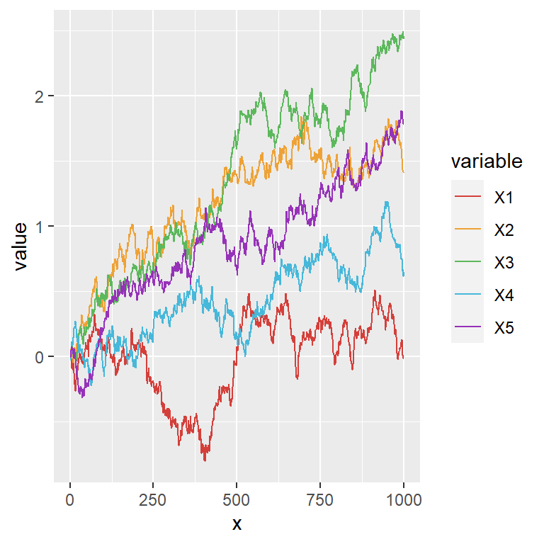
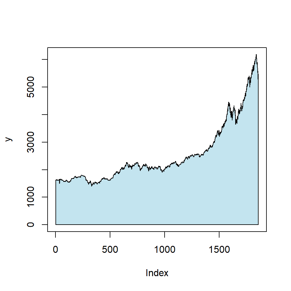
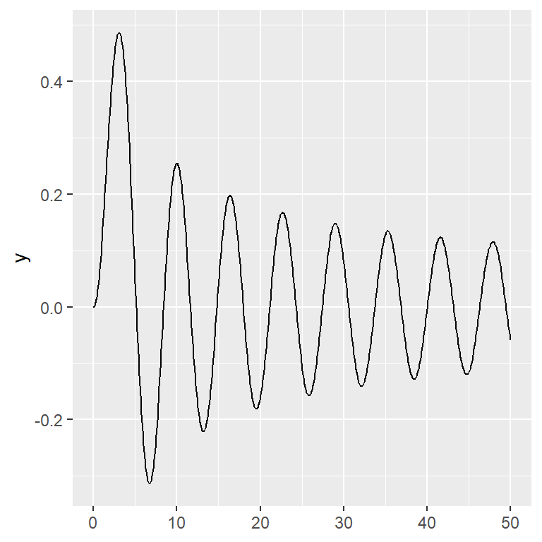
If you prefer static charts you can plot time series in ggplot2 and convert them into interactive charts with ggplotly. For financial data you can also create a candlestick chart.